Essential Statistics For AB Testing
Introduction#
In order to split test (or A/B test) a hypothesis efficiently, we need basic understanding of A/B testing statistics. While there so many notable articles out there on internet which are either too simple or extremely complex to apply in our optimization program. The objective of this article is to present the basic concepts of A/B testing statistics with examples in a precise manner that can be easily applied by Optimization Analysts.
So What is A/B testing to begin with ?#
As per Wikipedia - A/B testing (also known as bucket tests or split-run testing) is a randomized experiment with two variants, A and B. It includes application of statistical hypothesis testing or “two-sample hypothesis testing” as used in the field of statistics. A/B testing is a way to compare two versions of a single variable, typically by testing a subject’s response to variant A against variant B, and determining which of the two variants is more effective.
A/B test is basically an example of statistical hypothesis testing - Wherein two sampled data sets are compared against each other in order to validate if hypothesis yield statistically significant results or not. In practical terms an hypothesis is made to improve the conversion rate between Default (Control) and Variation experiences. The sample data collected from both experiences is used to determine if variation data set has statistically significant improvement over default.
Establishing Difference between Sampling and Population#
Population can be defined as including all people or items with the characteristic one wishes to understand. Because there is very rarely enough time or money to gather information from everyone or everything in a population, the goal becomes finding a representative sample (or subset) of that population.
Sampling is the selection of a subset (a statistical sample) of individuals from within a statistical population to estimate characteristics of the whole population. Two advantages of sampling are lower cost and faster data collection than measuring the entire population. Sample is basically a smaller portion of whole population data set used for calculations.
Understanding concept of Conversion Rate and Variance#
The Conversion Rate is basically the percentage of visitors that complete a desired goal (like purchase or lead submission). In simple terms it is calculated as (conversion/visits) x 100. For example: If your site has 1000 visitors and 10 complete purchase our conversion rate comes out to be (10/1000)*100 = 1%
The average conversion rate (mean) from a sampled data set is generally considered exact as populations conversion rate, for example since our conversion rate is 1% - One out of every 100 visitors sampled data set one will make purchase. (Which is not ideal calculation - Since more than one person can make purchase in first 100 visitor data and similarly effect other data sets as well). The table below illustrates the variance in conversions per sampled data set.
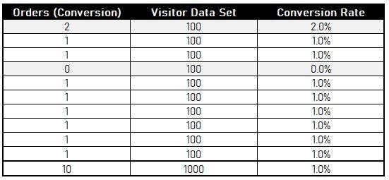
The conversion# will vary per 100 visitor sampled data set which in turns average out to be 1%, while the conversion rate per sampled data set could vary.
Standard Deviationmeasures how far a set of numbers are spread out from their average (mean) value. It is square root of variance. </bVariance is defined as average of squared difference from the mean. Standard Deviation can easily be calculated by using excel function STDEVwith conversion data set. The standard deviation for our orders data set is 0.47 (rounded two decimal places).
Insight on Confidence Interval and Margin of Error#
The conversion rate for the data set above is 1%, however it would not employ the confidence interval to our calculation since 1% is basically average (mean) conversion rate for our data set.
Margin of Error typically demonstrates how many percentage points our results will differ from real population conversion rate since we are always working with sample data sets. It is range of values below and above our sample data set averages in a confidence interval.
MOE can be calculated as [Critical Value x Standard Deviation] The Critical Value for 95% Confidence Interval is [1.96] (Refer - https://www.statisticshowto.datasciencecentral.com/probability-and-statistics/hypothesis-testing/margin-of-error/). MOE => 1.96 x 0.47 = 0.92 So basically ±0.92% is margin of error and gives us confidence interval spamming 0.8% - 1.92%
The upper bound of confidence interval is derived by adding margin of error to mean, similarly the lower bound is calculated by subtracting margin of error by mean.
Confidence Level can be set to whatever we require for analysis, however if we aim to achieve 99% certainty we would require significantly larger amount of sample data set which would require a test to run for very long duration.
The confidence level of 95% or 90% are frequently used by analyst as they have appropriate accuracy over realistic test duration.
I hope this article was able to breakdown complex statistical methods into simple use-cases and can be applied easily into optimization programs. If you enjoyed this post, I’d be very grateful if you’d help it spread by sharing it on Twitter/LinkedIn. Thank you!.